To help us provide you with free impartial advice, we may earn a commission if you buy through links on our site. Learn more
Question: I have a chart in Excel that shows my monthly expenses total for the last twelve months. The figure for each month is added to a column containing the previous amounts, like this:
| Month | Amount |
| Nov 13 | 233.12 |
| Dec 13 | 276.48 |
| Jan 14 | 229.76 |
| Feb 14 | 197.33 |
| Mar 14 | 213.22 |
| Apr 14 | 257.40 |
I need to automatically select the most recent twelve months, but obviously the range changes from month to month. How can I make the data range for my chart dynamic?
Ross Taylor
Answer: Making Excel work with dynamic ranges in charts is extremely fiddly, but it can be done. The first thing to do is to set up a dynamic range. To create a dynamic named range, on the Formulas menu choose Define Name. If you’re using an earlier version of Excel than 2010, you’ll find this option on the Insert menu under Names, Define. Either way, make sure the Define Names dialog appears. You now need to a dynamic range for the expense amounts. To do this you enter a formula into the Refers to box, and a name for the range into the New Name box.
The formula you’re going to enter uses the Offset function, which returns a reference to a range that is a specified number of rows and columns from a cell or range of cells. The reference that is returned can be a single cell or a range of cells. The Offset function has the format, ‘OFFSET(reference, rows, cols,
[height]
,
[width]
)’.
The reference is the ‘base’ cell from which you want to return the offset. Rows is the number of rows, up or down, that you want the upper-left cell to refer to, and cols is the number of columns, to the left or right, that you want the upper-left cell of the result to refer to. Height is the number of rows that you want the returned reference to be, and width the number of columns wide.
So if you want to pull out twelve rows of the expenses amounts from column B, where the numbers start in B1, you’d use, ‘=OFFSET($B$1,COUNTA($B:$B)-1,0,-12,1)’.
In addition to Offset, this formula contains two other items you might not be familiar with. Counta returns the number of cells that are not empty in a range, so, ‘COUNTA(A2:A23)’ would return 10 if there were 10 cells in the range A2:A23 that contained data.
You may also not be that familiar with the use of $B:$B as the range for the Counta function. While it’s more usual to include a row number as well as a column letter, you can miss the row number out and Excel will assume you want to look at the whole column, so ‘COUNTA($B:$B)’ counts the whole of column B.
You need to make this an absolute reference using the $, otherwise Excel alters the range reference as the formula is calculated. The tricky part here is that you have a title in your data, so you want to get the count of the cells with data in the entire column, minus the one header, hence, ‘COUNTA($B:$B)-1’.
You don’t want to move any columns to the left or right, so the column offset is 0. Next, we want the number of rows to be returned. You want the most recent 12 rows from the bottom, so -12 rows backwards, and you want it to be 1 column wide.
Once you’ve entered the formula into the Refers to box (changing the column location so it points to the data in your workbook), click OK to close the dialog box and save the named range. Repeat the process to get a named range for the months or any other data you want to use in your graph.
Now you can create the chart. This is fiddly, and if you don’t follow the steps exactly you’ll end up with Excel complaining about your references or turning the named range to a specific cell range reference.
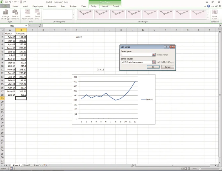
Create an empty chart by going to the Insert tab of the Office ribbon, and choosing a line chart from the options on offer. You’ll get a blank chart, and the Chart Tools contextual ribbon. Click on it, and in the Data group on the Design tab, click the Select Data button. The Select Data Source dialog box will appear. DO NOT enter anything into the Chart Data Range box. Instead, click the Add button in the Legend Entries (Series) section. The Edit Series dialog will appear. In the Series Values field enter the range name you created earlier, including the workbook name. In our case, the workbook is called bh319.xlsx, and the named range is expamounts, so we’d enter, ‘=bh319.xlsx!expamounts’.
If you use this method, Excel accepts the dynamic range in the chart, and when you change the range, the chart will be changed.