To help us provide you with free impartial advice, we may earn a commission if you buy through links on our site. Learn more
If you want a spreadsheet that has consistent values entered into it, you need to use Excel’s data validation too. This gives you a drop-down menu in a cell, only letting people enter a set range of inputs. We’ll show you how to use it, creating a home inventory spreadsheet along the way, although the techniques can be applied to any spreadsheet.
1 SET UP YOUR RANGE OF VALUES
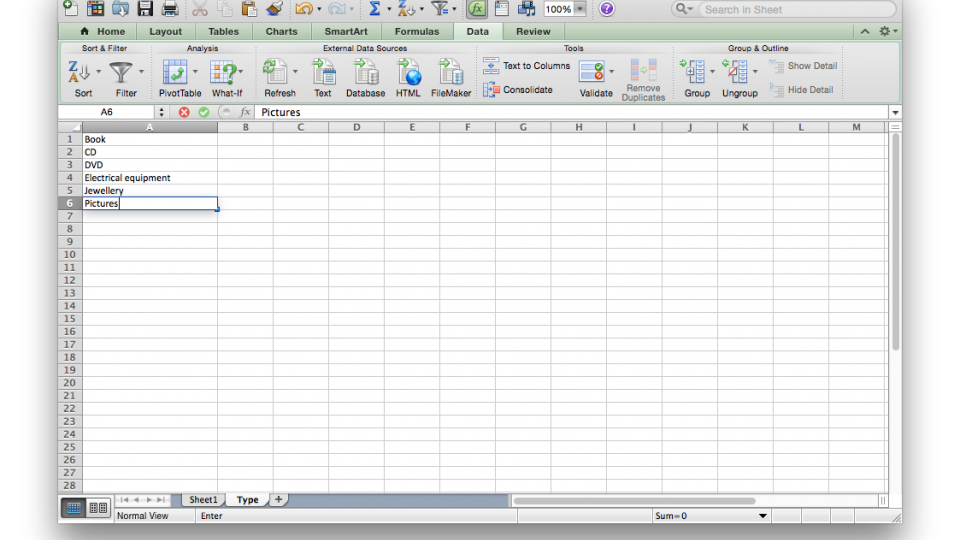
Create a new spreadsheet and click the plus button at the bottom of the window to create a new tab. Right-click the tab and select Rename, then enter a name for this tab (we’ve got with Type). Starting in cell A1 and moving to cell A2, then A3 and so on, enter the values that you want to appear in the drop-down menu. For our spreadsheet, we’ve gone with categories of item in the house (CD, DVD, Book, Electrical equipment and so on). Don’t worry if you forget something, as you can add it later. Click A to select the entire column and click Sort to sort your list alphabetically, making it easier to select a value. Not that you don’t need to create this list in a new tab (it can be created anywhere in the spreadsheet), but we like the way that it keeps everything neat.
2 SET UP YOUR SHEET
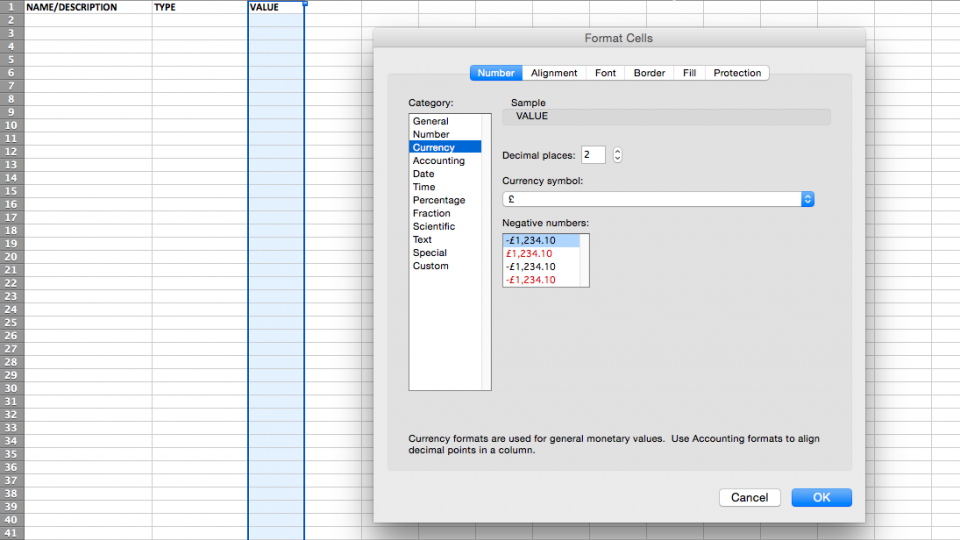
Click on Sheet1 to go back to the main sheet. In cells A1, B1 and C1, we’ve entered the headers ‘Name/description’, ‘Type’ and ‘Value’ respectively. We’ve also used Bold to make them stand out. To make the value column display everything in pounds (£) click C to select the entire column, right-click and select Format cells. Click the Number tab and select Currency and make sure that it’s set to £ and click OK.
3 SET UP VALIDATION
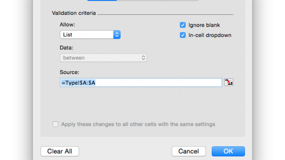
To set up your validation click column B, click the Data tab and click Validate. From the Allow menu select List (the other options let you restrict entry by setting limits for dates, numbers, text length and so on, but don’t give you a drop-down menu). Click the icon next to the Source entry box and then, in your spreadsheet, click the Type tab (or whatever you called your second tab) and click the A to select all of your data. You can just select the list items, but if you want to grow the list later you’ll need to repeat this step to include the new entries. Hit Enter to confirm and then click OK. At the moment, you’ve also got validation turned on for the cell header, which you don’t want. Click B1, click Validate and select ‘Any value’ from the Allow menu, then click OK.
4 START ENTERING DATA
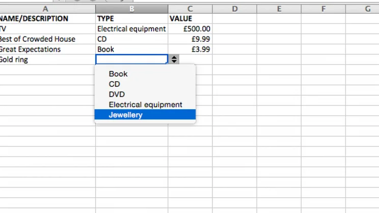
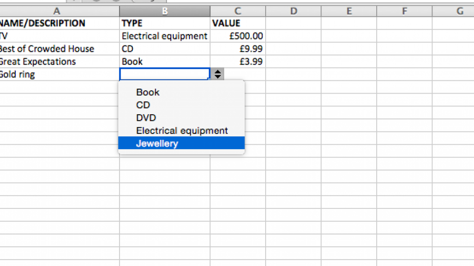
You can now start entering data into your spreadsheet. You’ll notice that when you click on a cell in column B that you get a drop-down menu, which only lets you enter data from the list you input into the second tab of your spreadsheet. Excel will not let you enter any other data.
5 GROWING THE VALIDATION LIST
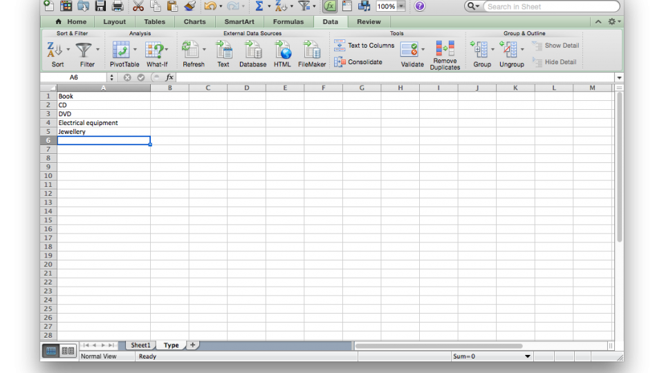
If you want to add anything to your validation list, just click on the second tab and enter a new value. Don’t forget to sort the list again, so that your values are easy to find. Finally, if you delete a value or change the spelling of one, your first spreadsheet will not update automatically and you’ll need to make the change manually. This tip works as we selected an entire column for validation; if you selected only your values, you’ll need to go back to Step 3 and reselect all of your new list.