To help us provide you with free impartial advice, we may earn a commission if you buy through links on our site. Learn more
With Excel’s Sumif function, you can add up the values of cells based on whether they match a given criteria. This helps you organise and compare values, helping you make sense of lots of information in an easy-to-digest manner. We’re using our house inventory spreadsheet, which we first created in our how to use validation in Excel article, and then updated in our how to use countif in Excel guide. We’ll use Sumif to add up the value of each product category, although the instructions can easily be modified for any spreadsheet.
1 SETUP TABLE FOR COUNTIF
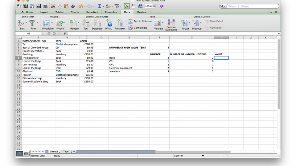
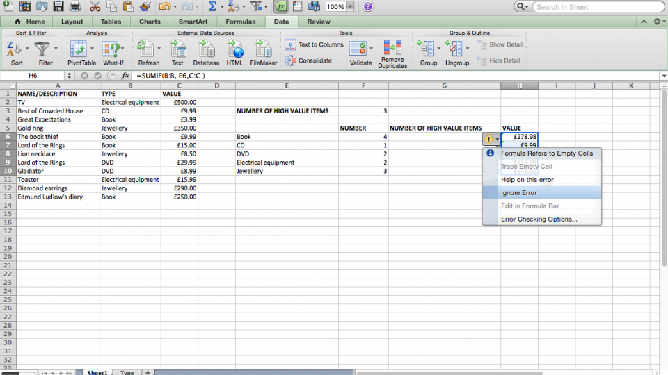
Our summary table is already set up to display the number of each item and the number of high value items. We’ll just add a new column to contain the total value of all products in that category. In Cell H5 just enter ‘Value’ and hit Enter.
2 CREATE THE FIRST SUM
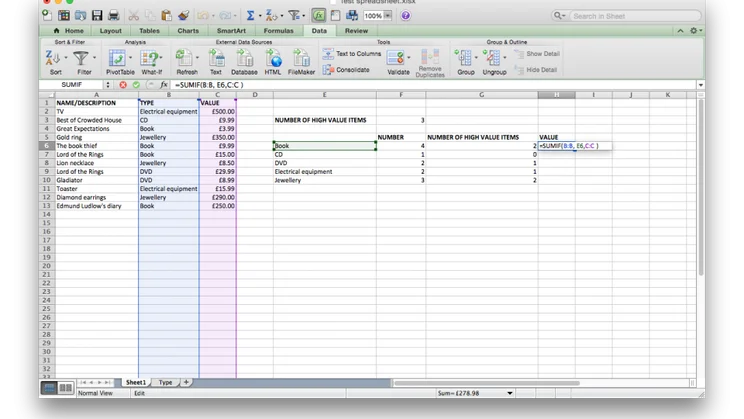
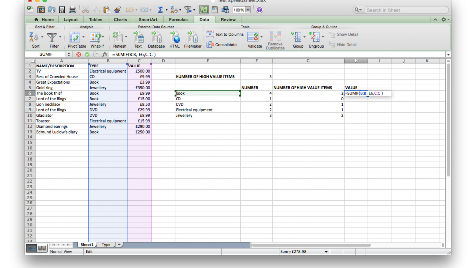
Sumif is very similar to the Countif function, although it has one extra parameter to it. The function looks like this: sumif(<range>, <criteria>, <sum range>). The first to parameters are the same as for Countif and specify which range of cells to look at and the value that they should match. The last parameter is the range of cells to add up. In our spreadsheet, in Cell H6, we’d use the function, =sumif(B:B, E6, C:C). This searches column B (our ‘Type’ column) for entries that match E6 (‘Book’ in our example). For any hit on column B, Excel looks along the same row and adds the value from column C into a running total. So, if B2 matches the search, Excel adds the value from C2 to a running total and so on down through the entire search range.
3 FORMAT AND COPY DOWN
Your new formula only spits out a number, so right click Cell H6 and select Format Cells, then click Currency and click OK. You can now drag the formula down to encompass all categories in your spreadsheet. Click Cell H6, click and hold the square box at the bottom-right of the cell and drag down to the bottom of the list. Again, Excel will warn you that the formula is looking at empty cells, so select them all, click the exclamation icon that appears and select Ignore error.
4 SELECTIVELY SUM
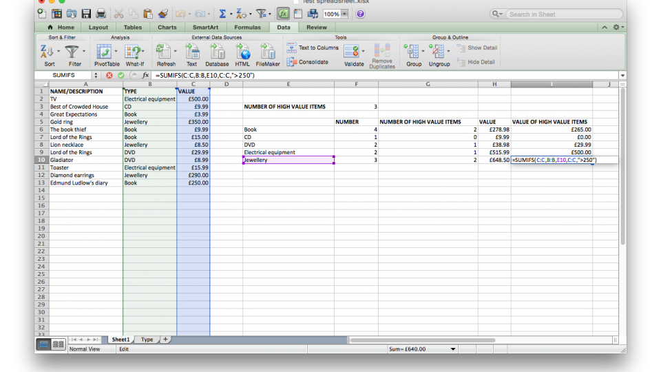
If you want to apply a sum to a subsection of your criteria, you can do that easily using the Sumifs function. For example, in our spreadsheet we may want to selectively add up the value of our high value items as well. Create a new header in cell I5 and enter ‘Value of high value items’.
Sumifs works like this: Sumifs(<sum range>, <range1>, <criteria1>, <range2>, <criteria2>, and so on. In other words, you only get a sum when all of the criteria for all of the ranges are met.
In our example, to add up the value of all high value books, we’d use the formula, =sumif(C:C, B:B, E6, C:C, “>10”). This says, only add up the value if the Type column (B:B) is a Book (E6) and the value (C:C) is greater than £10 (“>10”). You can format the cell to display currency, copy it down to fill in the list and adjust the “>10” part to match what you consider a high-value item is for each category.